library(tidyverse)
add_numbers <- function(x, y) {
x + y
}
starwars |>
mutate(my_product = add_numbers(mass, height), .after = mass)Functions in R
R is a functional programming language.1 This means repetitive execution is emphasized without using FOR loops.2 No FOR loops‽ How is that possible? Basically, coders focus on applying the same operation, row by row, over a data frame — without toiling over the syntax of For loops.
If you’re new to R, you may not realize that you’ve been using functions throughout this workshop series. All the packages we introduced (dplyr, ggplot2, skimr, and even base-R, etc.) are made up collections of functions. For example, {dplyr} gives us the filter() and the select() functions. At the end of the section on regression, we saw an example of using the nest() function so our data frame is set for the repetition of our regression (the lm() function) row-by-row. We did this without ever writing a FOR loop.
Definition
Functions
Blocks of code that can be invoked by the coder to perform fundamental steps.
Functions can accept inputs and yield outputs. If we put a string of functions together we have a more complex function. We may want to apply this complex function to some group of data till we reach the end. In R the basic syntax of a function looks like this
```{r}

# Define function to add two numbers
add_numbers <- function(x, y) { x + y }

```
Then we can call that function like this
```{r}
add_nubmers(8, 10)
```
The console will return a response, or we can store that response in an object. Or we can combine that function with the mutate function and iterate over all the rows in a data frame
While the custom function, add_numbers, didn’t save us much time. We can create more sophisticated functions. For example, we can write a function that plots x and y.
The function, below, uses indirection syntax (i.e. double-braces) because there’s a difference between an environment variable and a data variable. An explanation of indirection is found in the enthusiastically recommended Programming with dplyrvignette. Essentially, an environment variable shows up in the RStudio environment tab. While a data variable is the name of a variable within an environment variable. For example, in a data frame, a column header variable name is a data variable. Data variables have to be called with the embrace operator {{so that they data can be referenced indirectly. This indirection overcomes a data masking feature which allows for more efficient coding in many cases.
Essentially, ease of coding is emphasised with data masking. This data masking makes it easier to learn R. As a beginner there are fewer syntactical barriers when coding in a tidyverse context. The paradox of this early simplicity comes at the cost of more complex syntax when composing complex functions. This syntactical complexity occurs because data-masked variables need to be referred to indirectly.
make_scatterplot <- function(my_df, my_x, my_y, my_color) {
my_df |>
drop_na() |>
ggplot(aes(x = {{my_x}}, y = {{my_y}})) +
geom_point(aes(color = {{my_color}})) +
geom_smooth(method = lm, se = FALSE, formula = y ~ x)
}
make_scatterplot(starwars, height, mass, gender)
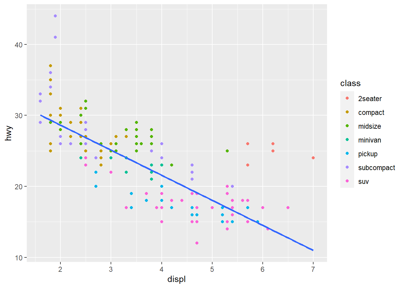
make_scatterplot(mpg, displ, hwy, class)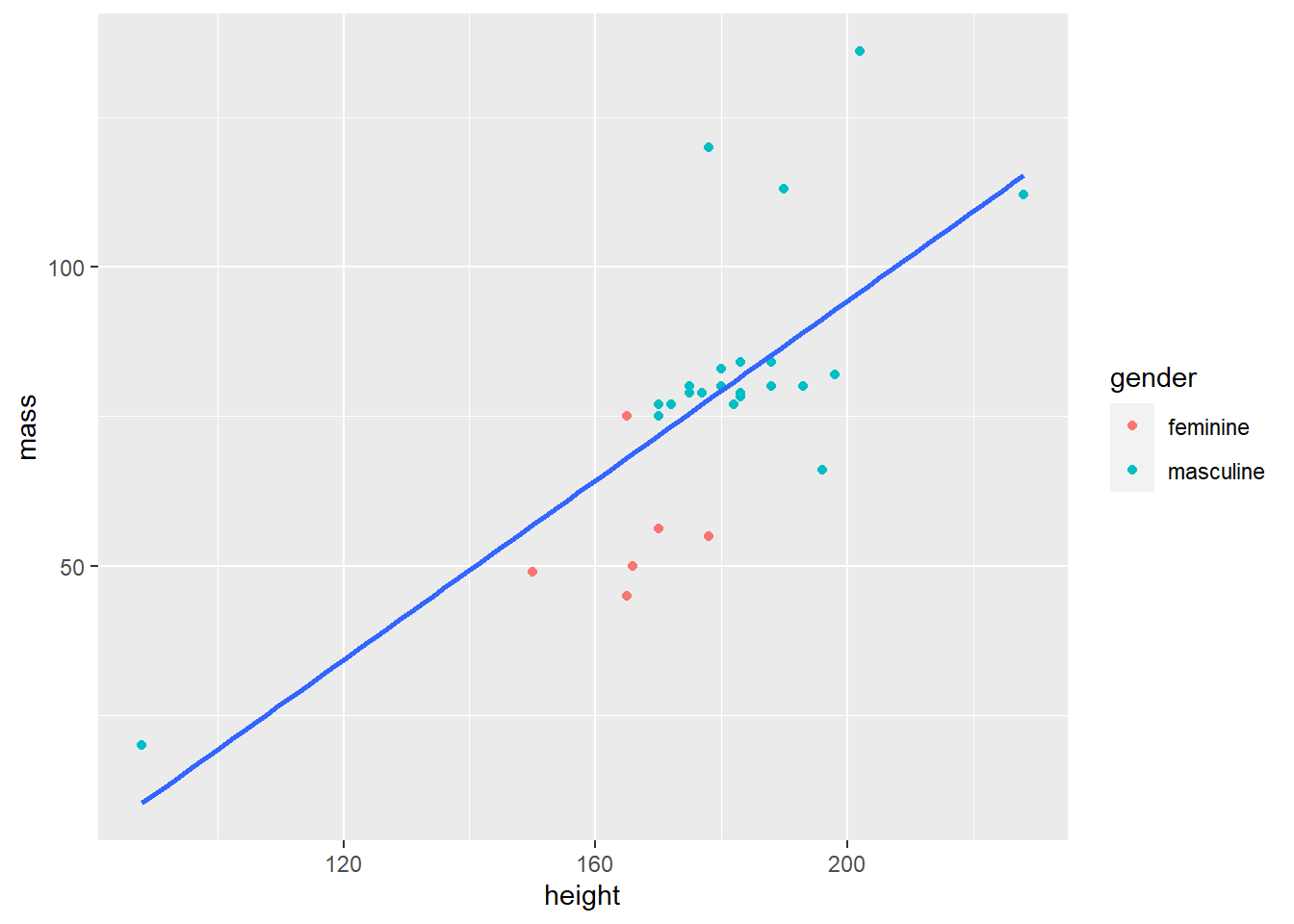
Rule of thumb
If you have to write the same code three times or more, write a function. Among the advantages, this prevents typographical errors. Additionally, writing functions can prevent mistakes in coding because there will be fewer places to update.
Can it be simpler?
In a word, yes, but there may be limitations. In the section on pivoting data, we saw how pivoting data to the tall format made it easier to generate multiple {ggplot2} plots. We combine pivoting with the facet_wrap() function to visualize multiple plots with minimal coding. While we didn’t write a special custom function, we did use the functional programming approach to iterate over rows of a data frame. Without pivoting the data and faceting the plots, this code might have taken ten-times as much code, most of it repetitive and all of it susceptible to typing mistakes.
inc_levels = c("Don't know/refused",
               "<$10k", "$10-20k", "$20-30k", "$30-40k",
               "$40-50k", "$50-75k", "$75-100k", "$100-150k",
               ">150k")

relig_income %>%
  pivot_longer(-religion, names_to = "income", values_to = "count") %>%
  mutate(religion = fct_lump_n(religion, 4, w = count)) %>%
  mutate(income = fct_relevel(income, inc_levels)) %>%
  summarise(sumcount = sum(count), .by = c(religion, income)) %>%
  ggplot(aes(fct_reorder(religion, sumcount),
             sumcount)) +
  geom_col(fill = "grey80", show.legend = FALSE) +
  geom_col(data = . %>% filter(income == "$40-50k"),
           fill = "firebrick") +
  geom_col(data = . %>% filter(income == ">150k"),
           fill = "forestgreen") +
  coord_flip() +
facet_wrap(vars(income), nrow = 2) 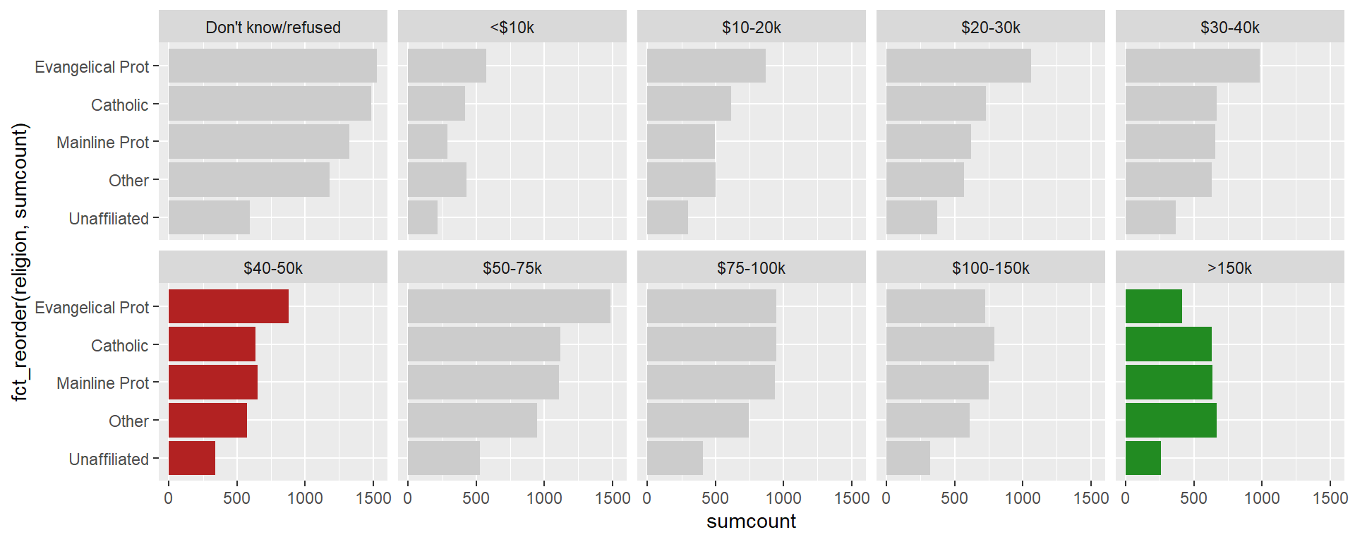
Mapping over a data frame
But how do we apply functions, row-by-row, over a data frame without using FOR loops? Move to the section on iteration with {purrr}