library(moderndive)
library(broom)
library(tidyverse)

evals |>
  janitor::clean_names() |>
nest(data = -gender)Iteration with {purrr}
Review the functions page!
If you have not already read the functions page, do so before reading about {purrr}. The purrr package is about applying functions repetitively. You should have a good idea about what a function is and how to write a custom function.
From the functions page we learned scant definitions of functional programming and functions. We also learned about the special conditions of programming with {dplyr}, which demands a working understanding of environment and data variables.1 Now we want to apply our functions, row-by-row, to a data frame. We’ll use the purrr package.
Rule of thumb
Never feel bad for using a FOR loop.
Remember that in functional programming we’re iterating, or recursing, without using FOR loops. For example, in the regression page, we saw an example of nesting data frames by category (i.e. by gender). After nesting, we have two subsetted data frames that are embeded within a parent-data-frame. The embedded data frames are contained within a list-column.
nest()
We can subset by gender, creating two new subset data frames that we’ll put in a new column with the variable name: data. This subsetting is accomplished with the nest() function.
map()
Using {purrr} we can apply a function — such as a linear model regression lm() — over each row of the parent data frame. To do this, we use the map_ class of functions. I say class of functions, because purrr::map_ allows us to define the data-type2 returned by the mapped function. For example, sometimes we want to return a character data-type (map_chr), sometimes an integer (map_int), sometimes a data frame (map_df), etc. In the case of a linear model, which is a list data-type, we’ll use the generic map() function to apply an anonymous function.
Anonymous functions
Examples of an anonymous function:
\(x) x + 1
function(x) x + 1
Unlike the add_numbers() function we composed on the functions page, anonymous functions have no object name. Hence they are anonymous. Anonymous functions, sometimes called lambda functions, are a convenience for coders using functional programming languages.
my_subset_df <- evals |>
  janitor::clean_names() |>
  nest(my_data = -gender) |>
  mutate(my_fit_bty = map(my_data, function(my_data)
                                lm(score ~ bty_avg, data = my_data)
                         )
        )
my_subset_df
Look at the fitted object
When we look at the resulting my_fit_bty data variable, we see the kind of output we get from lm()
my_subset_df$my_fit_bty[[1]]
Call:
lm(formula = score ~ bty_avg, data = my_data)
Coefficients:
(Intercept) bty_avg
3.95006 0.03064
[[2]]
Call:
lm(formula = score ~ bty_avg, data = my_data)
Coefficients:
(Intercept) bty_avg
3.7666 0.1103 Earlier, we learned to use the broom::tidy() function to transform a fitted model — contained as a list data-type — into a data frame.3 For example, we can easily tidy the first model which coerces the list data-type into a data frame.
tidy(my_subset_df$my_fit_bty[[1]])Named functions
If we wanted to tidy all the models — not only the fist model (above) — then we use the map function (again.) This time we map a named function, i.e. broom::tidy(). We do this row-by-row with map(), i.e. without using a FOR loop.
my_subset_df |>
  mutate(my_fit_bty_tidy = map(my_fit_bty, tidy))
A difference between my_fit_bty and my_fit_bty_tidy is that my_fit_bty_tidy is the model output for the former is a list, the later is a data frame. Therefore, the parent data frame — my_subset_df— has a data variable: my_fit_bty_tidy, aka my_subset_df$my_fit_bty_tidy. my_fit_bty_tidy is a list-column of nested data frames, just like my_subset_df$data — which we nested in the first code-chunk of this page as evals$data.
To un-nest the data frames, use the unnest() function.
my_subset_df |>
  mutate(my_fit_bty_tidy = map(my_fit_bty, tidy)) |>
  unnest(my_fit_bty_tidy)
And now we have fitted model data, contained as tidy-data, within a data frame, which we can manipulate further with other tidyverse functions. For example, using dplyr functions it’s easy to make a pipeline to look at the p-values of bty_avg, by gender.
my_subset_df |>
  mutate(my_fit_bty_tidy = map(my_fit_bty, tidy)) |>
  unnest(my_fit_bty_tidy) |>
  select(gender, term, p.value) |>
  filter(term == "bty_avg")
When we combine linear modeling with other broom functions such as glance() and augment(), then we can build on our analysis and data manipulation.
Anonymous functions
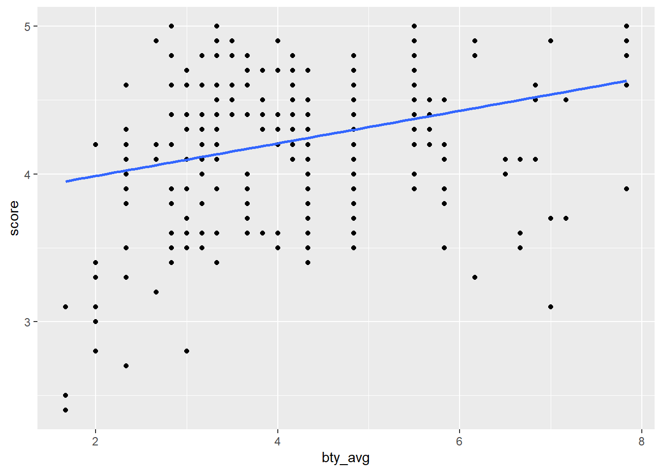
Anonymous functions have no name. Unlike a named function (e.g. broom::tidy above, or make_scatterplot from the functions page). Below we map an anonymous function within map(). The first argument to map is a list or data frame. The next argument can be a named function or an anonymous function. In the example below, the anonymous function produces a scatter plot with a regression line.
my_subset_df_with_plots <- my_subset_df |>
  mutate(my_plot = map(my_data, function(my_data)
    my_data |>
      ggplot(aes(bty_avg, score)) +
      geom_point() +
      geom_smooth(method = lm, se = FALSE, formula = y ~ x)
                      )
         )
my_subset_df_with_plots
And now we can pull those plots
my_subset_df_with_plots |>
  pull(my_plot)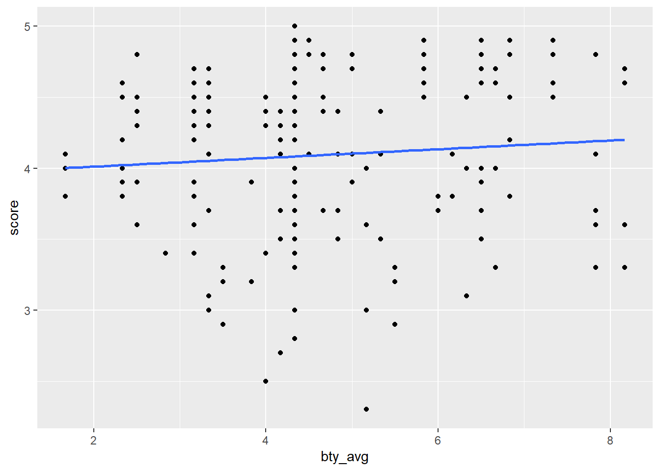
map2() & pmap()
If you have more than one argument to map, you can use functions such as map2() or pmap(). An example of map2() can be found on the regression page.
```{r}
# Example of mapping a anonymous function with two variables.

map2(my_df, my_plot, gender, function(x, y) { x + labs(title = str_to_title(y)) } )

# x refers to the second argument of map2, i.e. `my_plot`

# y refers to the third argument, i.e. `gender`

```
References
Wickham, Hadley, Mine Çetinkaya-Rundel, and Garrett Grolemund. 2023. R for data science : import, tidy, transform, visualize, and model data. 2nd edition. Sebastopol, CA: O’Reilly Media, Inc.
Footnotes
Links and footnotes on the functions page will lead to more detailed information on those topics.↩︎
A fuller explanation of data types can be found in R for Data Science (Wickham, Çetinkaya-Rundel, and Grolemund 2023)↩︎
Having our regression model wrapped as a data frame means we can use other {dplyr} functions to more easily manipulate our model output.↩︎