library(dplyr)
library(ggplot2)
library(moderndive)
library(broom)
library(skimr)Regression
Load library packages
Data
Data are from the {moderndive} package1, Modern dive (Kim, Ismay, and Kuhn 2021), and the {dplyr} package (Wickham et al. 2023).
evals_ch5 <- evals %>%
  select(ID, score, bty_avg, age)

evalsevals_ch5evals_ch5 %>%
summary() ID score bty_avg age
Min. : 1.0 Min. :2.300 Min. :1.667 Min. :29.00
1st Qu.:116.5 1st Qu.:3.800 1st Qu.:3.167 1st Qu.:42.00
Median :232.0 Median :4.300 Median :4.333 Median :48.00
Mean :232.0 Mean :4.175 Mean :4.418 Mean :48.37
3rd Qu.:347.5 3rd Qu.:4.600 3rd Qu.:5.500 3rd Qu.:57.00
Max. :463.0 Max. :5.000 Max. :8.167 Max. :73.00 skimr::skim(evals_ch5)| Name | evals_ch5 |
| Number of rows | 463 |
| Number of columns | 4 |
| _______________________ | |
| Column type frequency: | |
| numeric | 4 |
| ________________________ | |
| Group variables | None |
Variable type: numeric
| skim_variable | n_missing | complete_rate | mean | sd | p0 | p25 | p50 | p75 | p100 | hist |
|---|---|---|---|---|---|---|---|---|---|---|
| ID | 0 | 1 | 232.00 | 133.80 | 1.00 | 116.50 | 232.00 | 347.5 | 463.00 | ▇▇▇▇▇ |
| score | 0 | 1 | 4.17 | 0.54 | 2.30 | 3.80 | 4.30 | 4.6 | 5.00 | ▁▁▅▇▇ |
| bty_avg | 0 | 1 | 4.42 | 1.53 | 1.67 | 3.17 | 4.33 | 5.5 | 8.17 | ▃▇▇▃▂ |
| age | 0 | 1 | 48.37 | 9.80 | 29.00 | 42.00 | 48.00 | 57.0 | 73.00 | ▅▆▇▆▁ |
Correlation
strong correlation
Using the cor function to show correlation. For example see the strong correlation between starwars$mass to starwars$height
my_cor_df <- starwars %>%
  filter(mass < 500) %>%
  summarise(my_cor = cor(height, mass))
my_cor_df
The cor() function shows a positive correlation of 0.7612612. This indicates a positive correlation between height and mass.
weak correlation
By contrast, see here a regression line that visualizes the weak correlation between evals_ch5$score and evals_ch5$age
evals_ch5 %>%
  ggplot(aes(score, age)) +
  geom_jitter() +
  geom_smooth(method = lm, formula = y ~ x, se = FALSE)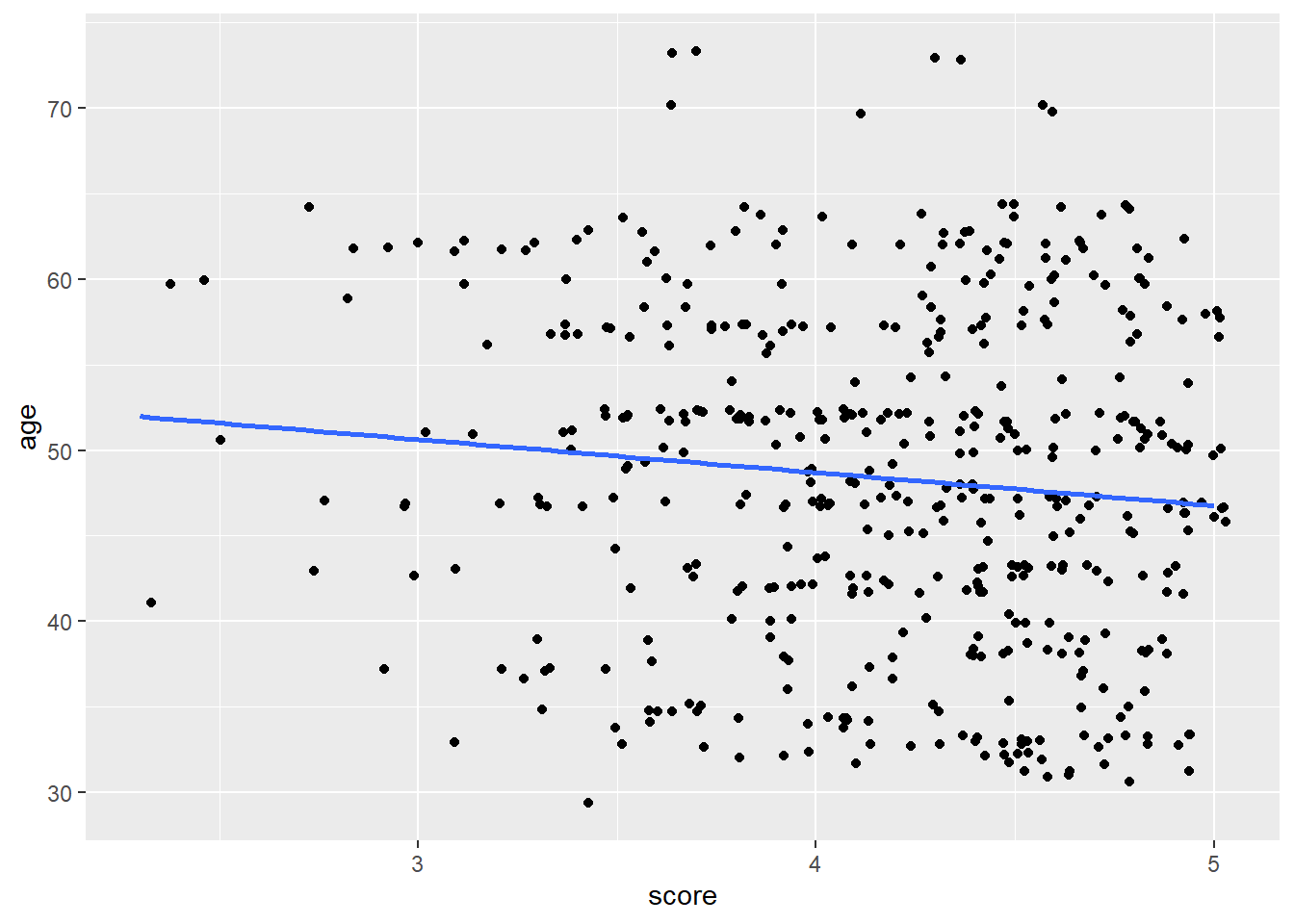
Linear model
Interpretation
For every increase of 1 unit increase in bty_avg, there is an associated increase of, on average, 0.067 units of score. from ModenDive (Kim, Ismay, and Kuhn 2021)
# Fit regression model:
score_model <- lm(score ~ bty_avg, data = evals_ch5)

score_model
Call:
lm(formula = score ~ bty_avg, data = evals_ch5)

Coefficients:
(Intercept)      bty_avg
3.88034 0.06664 summary(score_model)
Call:
lm(formula = score ~ bty_avg, data = evals_ch5)

Residuals:
    Min      1Q  Median      3Q     Max
-1.9246 -0.3690  0.1420  0.3977  0.9309

Coefficients:
            Estimate Std. Error t value Pr(>|t|)
(Intercept)  3.88034    0.07614   50.96  < 2e-16 ***
bty_avg      0.06664    0.01629    4.09 5.08e-05 ***
---
Signif. codes:  0 '***' 0.001 '**' 0.01 '*' 0.05 '.' 0.1 ' ' 1

Residual standard error: 0.5348 on 461 degrees of freedom
Multiple R-squared:  0.03502,   Adjusted R-squared:  0.03293
F-statistic: 16.73 on 1 and 461 DF,  p-value: 5.083e-05
Broom
The {broom} package is useful for containing the outcomes of some models as data frames. A more holistic approach to tidy modeling is to use the {tidymodels} package/approach
Tidy the model fit into a data frame with broom::tidy(), then we can use dplyr functions for data wrangling.
broom::tidy(score_model)get evaluative measure into a data frame
broom::glance(score_model)More model data
predicted scores can be found in the .fitted variable below
broom::augment(score_model)Example of iterative modeling with nested categories of data
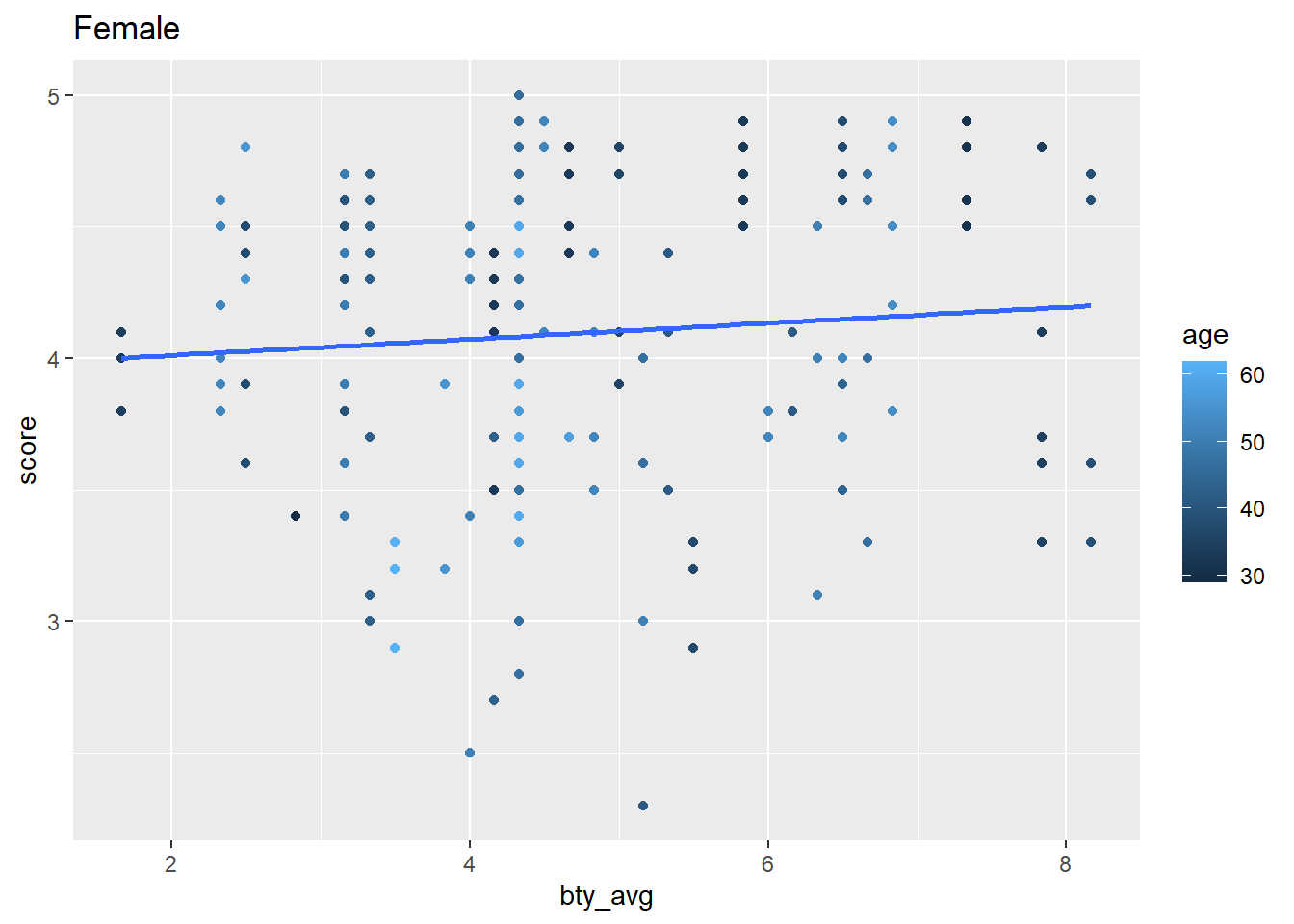
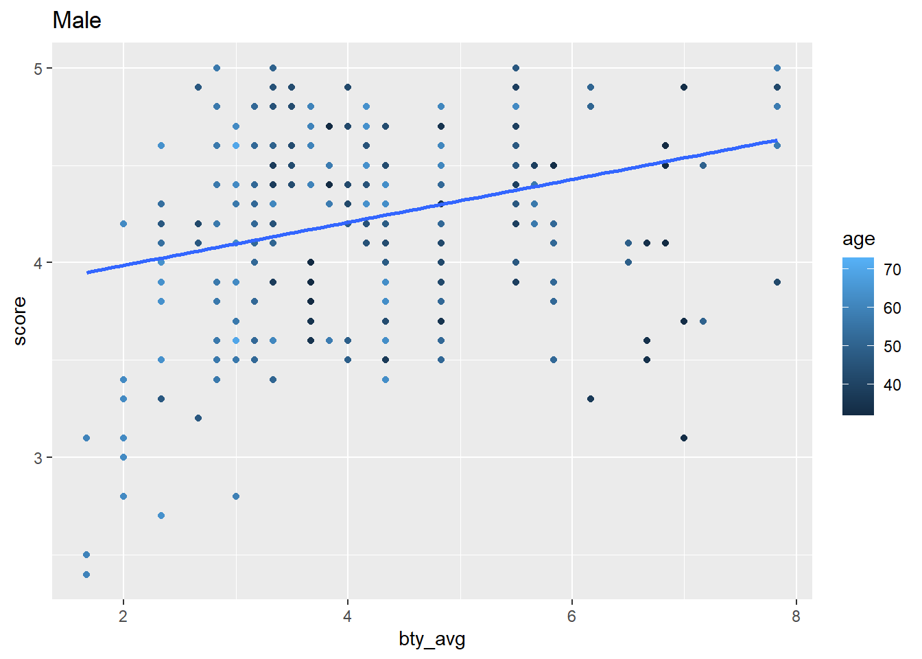
In this next example we nest data by the gender category, then iterate over those categories using the {purrr} package to map anonymous functions over our data frames that is nested by our category. Look closely and you’ll see correlations, linear model regression, and visualizations — iterated over the gender category. purr::map iteration methods are beyond what we’ve learned so far, but you can notice how tidy-data and tidyverse principles are leveraged in data wrangling and analysis. In future lessons we’ll learn how to employ these techniques along with writing custom functions.
library(tidyverse)

my_iterations <- evals |>
  janitor::clean_names() |>
  nest(data = -gender) |>
  mutate(cor_age = map_dbl(data, \(data) cor(data$score, data$age))) |>
  mutate(cor_bty = map_dbl(data, \(data) cor(data$score, data$bty_avg)))  |>
  mutate(my_fit_bty = map(data, \(data) lm(score ~ bty_avg, data = data) |>
                            broom::tidy())) |>
  mutate(my_plot = map(data, \(data) ggplot(data, aes(bty_avg, score)) +
                         geom_point(aes(color = age)) +
                         geom_smooth(method = lm,
                                     se = FALSE,
                                     formula = y ~ x))) |>
  mutate(my_plot = map2(my_plot, gender, \(my_plot, gender) my_plot +
                          labs(title = str_to_title(gender))))
This generates a data frame consisting of lists columns such as my_fit_bty and my_plot
```{r}
my_iterations
```
my_terations$my_fit_bty is a list column consisting of tibble-style data frames. We can unnest those data frames.
```{r}
my_iterations |>
  unnest(my_fit_bty)
```
my_iterations$my_plot is a list column consisting of ggplot2 objects. We can pull those out of the data frame.
```{r}
my_iterations |>
  pull(my_plot)
```
Next steps
The example above introduces how multiple models can be fitted through the nesting of data. Of course, modeling can be much more complex. A good next step is to gain basic introductions about tidymodels. You’ll gain tips on integrating tidyverse principles with modeling, machine learning, feature selection, and tuning. Alternatively, endeavor to increase your skills in iteration using the purrr package so you can leverage iteration with custom functions.
References
Kim, Albert, Chester Ismay, and Max Kuhn. 2021. “Take a Moderndive into Introductory Linear Regression with r.” Journal of Open Source Education 4 (41): 115. https://doi.org/10.21105/jose.00115.
Wickham, Hadley, Romain François, Lionel Henry, Kirill Müller, and Davis Vaughan. 2023. Dplyr: A Grammar of Data Manipulation.